
Risk-Adjusted Returns – Looking Beyond The Dollars
- Eng Guan

- May 20, 2022
- 6 min read
Updated: Apr 26, 2023
All industries have their fair share of jargon. It can be frustrating for a potential investor when he/she could not comprehend the investment manager, even when they speak a common language. If you have sat through any presentations by a hedge fund manager or read their monthly reports, you will most certainly have come across terms like Sharpe ratio, Sortino ratio, or Calmar ratio. What are these ratios? Yes, you probably have guessed it by now. They are risk-adjusted returns.
First, let us talk about absolute returns. Absolute returns of an investment are simply the dollar return of the investment. It is often expressed as a percentage. If I invest $1000 in a fund, and in a year, its value grows to $1200, then my absolute return for that year is $200 or 20%. This is what most people mainly focused on. After all, we invest with the ultimate aim to make money. However, absolute returns are only one part of the equation when assessing any investments. We cannot only look at returns in isolation without talking about risks and vice versa. Not all “returns” are equal. A risky investment generating a higher return is not necessarily better than one with a lower return but does so at a lower risk.
Taking Risk Into Account
So how can we take risks into account when we compare the performance of different investments? We can use returns per unit risk, instead of absolute returns. In this case, the risk becomes the common denominator across all investments considered. Each of the ratios mentioned uses a specific risk measure. Sharpe ratio uses volatility, Sortino ratio uses downside volatility, and Calmar ratio uses maximum drawdown.
Risk is a very complex subject. There is a broad range of risks and some cannot be adequately quantified. Many people also questioned the validity of volatility-based measures as a proxy for risks. But we can discuss this another time. For now, let’s just look at how these risk measures and ratios work.
Volatility – Mathematical Interpretation
Volatility appears in modern portfolio theory. It has gained wide acceptance and many funds use it as their proxy for risk. You can view it as a measure of the tendency of the fund’s value to swing up and down. The larger those swings are, the more volatile the fund is. Because of that, we are more uncertain whether the fund is going to meet its return target, and hence the riskier it is.
For the mathematically inclined, the volatility of a fund’s return is basically its standard deviation. Standard deviation quantifies the dispersion of the returns around its mean.
Most funds calculate annualized volatility as follows (assuming monthly return data)
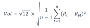
Where
n is the total number of months
Rt is the return on investment in month t
RM is the average monthly return on investment over the entire period
Firstly, we get the variance using the squared difference between each month’s return and the average monthly return over the entire period. Then we scale it by a time factor of 12 to get the annualized variance. Finally, we apply a square root to the number to arrive at the annualized volatility. While this formula might look a bit daunting, you can easily calculate this in excel using the STDEV() formula on the return series.
Volatility – Visual Interpretation
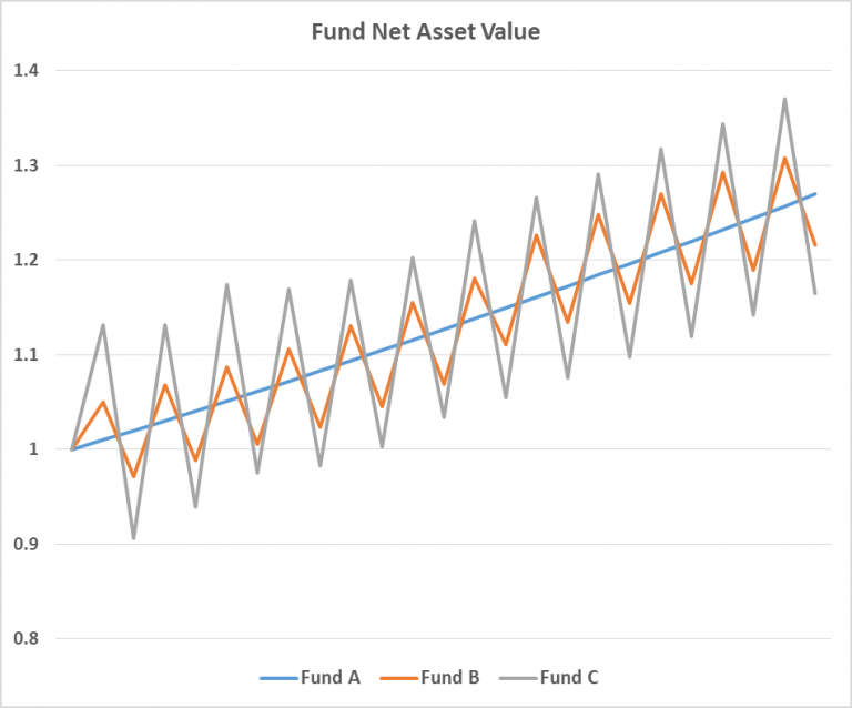
This diagram is a simple illustration of the concept of volatility with 3 funds A, B, and C. To accentuate the idea, I deliberately made the swings appear even and non-random. But do note that this does not resemble anything in the real world.
Fund A has zero volatility. It appreciates in a straight line at a constant rate. Fund B has medium volatility. It swings up and down gently. Fund C has high volatility. It makes big swings both ways.
Downside Volatility
You might have noticed by now that volatility does not care whether the fund makes or loses money. It penalizes both upside and downside as long as they deviate from the mean. But upside volatility is in fact good for us. So why are we punishing the fund for performing above its expected average return? This raises a question. If our concern is losing money, then shouldn’t we look only at deviations below the expected return or downside volatility?
Mathematically, we can express downside volatility as
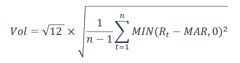
Where
n is the total number of months
Rt is the return on investment in month t
MAR is the Minimum Acceptable Return.
The Minimum Acceptable Return is a user-defined parameter. This is often set to zero. It effectively means that I am flushing all positive returns to zero while keeping the negative returns to compute the downside volatility.
Maximum Drawdown
Maximum drawdown is the simplest among the 3 risk measures here. It is the largest historical loss you can experience based on the peak-to-trough NAV of the fund. This occurs when you buy and sell at the worst possible time. Well, shit does happen.
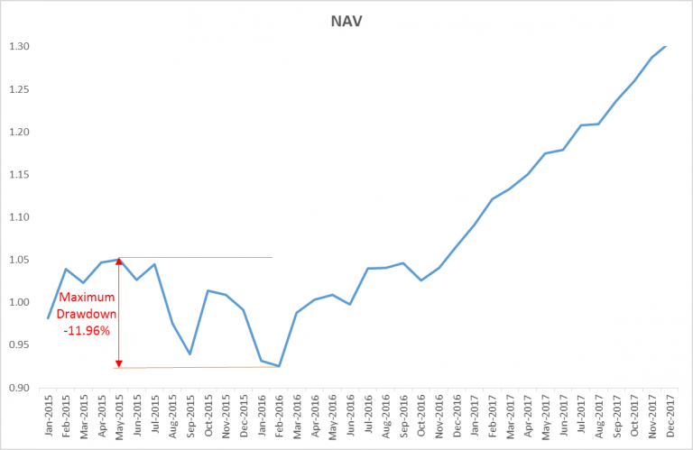
Using the returns, we can construct the NAV of the fund assuming it begins at a value of 1. Basically, there is a drawdown only when the fund is below its previous high. When the fund rallies and make a new high, there will be no drawdown i.e. drawdown is 0%.
The diagram below shows the deepest drawdown or peak to trough in the NAV of the fund. So in the worst scenario, an investor who had invested in the fund will lose at most 11.96%. But of course, this is based on historical data and does not mean that the fund will never exceed this drawdown in the future.
The second diagram is a drawdown plot. It clearly shows you where the different drawdowns are and how long the fund took to get out of these drawdowns (i.e. when the drawdown goes back to zero).

The 3 Risk-Adjusted Returns – Sharpe, Sortino, Calmar
We are now ready to compute the 3 ratios.
Sharpe Ratio
Sharpe ratio was first conceived by Nobel Laureate William F. Sharpe in 1966 and further revised for use by the fund industry. While there are other measures around, Sharpe Ratio is now the de facto standard when the industry talks about risk-adjusted returns. It uses volatility as the common denominator.

Many funds may set the risk-free rate to zero in their performance reports. This simplifies matters and applies a common yardstick across all funds. Intuitively, if Fund A has a higher Sharpe Ratio than Fund B, then Fund A is better at extracting returns according to this measure. It delivers more return per unit risk taken. This is somewhat similar to measuring a worker’s productivity. If Worker A produces more output in an hour than Worker B, then Worker A is more productive than Worker B.
Sortino Ratio
Harry Markowitz is the first to suggest the idea of using only downsides to measure risk, but it was Dr Frank Sortino who came up with the formula for the Sortino ratio. It is essentially a modification of the Sharpe ratio. The difference is the use of downside volatility as the denominator and a Minimum Acceptable Return as the target return.

Calmar Ratio
The Calmar ratio was developed by Terry W. Young. Yes, that is right. It is not by someone called Calmar. It is based on the name of his company newsletter instead. This ratio is computed using 36 months of data i.e. the annualized return and the maximum drawdown over the past 36 months.

Because Calmar is based on maximum drawdown, this ratio tends to be more stable than Sharpe or Sortino. Most of the time, it is the numerator that changes.
Final Points
When it comes to applying the ratios to assist in performance evaluation, there is no hard and fast rule as long as you enforce a fair and consistent principle. For example, while Calmar is defined to be calculated over 36 months, there is no rule stopping you to extend the period as far back as inception. Although of course, you might end up with a maximum drawdown figure that has not changed for the past 2 decades. This might draw questions on how relevant the figure is in today’s context. And even though there is no risk-free rate in the equation, adding it in does not do you any harm either. The situation is similar for Sharpe and Sortino.
However, you might want to note that assessing a fund’s performance goes much beyond just looking at a few ratios. There are many other quantitative metrics that academics and industry have come up with. Statistical measures, while useful, are also only one part of the equation when analyzing a fund or any other investments. The qualitative aspects such as the fund’s philosophy, strategy, mandate, portfolio managers, risk management methodologies, etc. are equally important and should be given serious focus when doing any due diligence.


Comments